Study-area layouts
The study-area figure — country → region → detail, with connecting lines and a highlighted focus area — is the signature research map. AcadGIS builds the whole thing in one call.
import acadgis as agis

agis.study_area(
    "Bangladesh",
    steps=[("division", "Dhaka"), ("district", "Madaripur")],
    template="cascade", terrain=True,
)
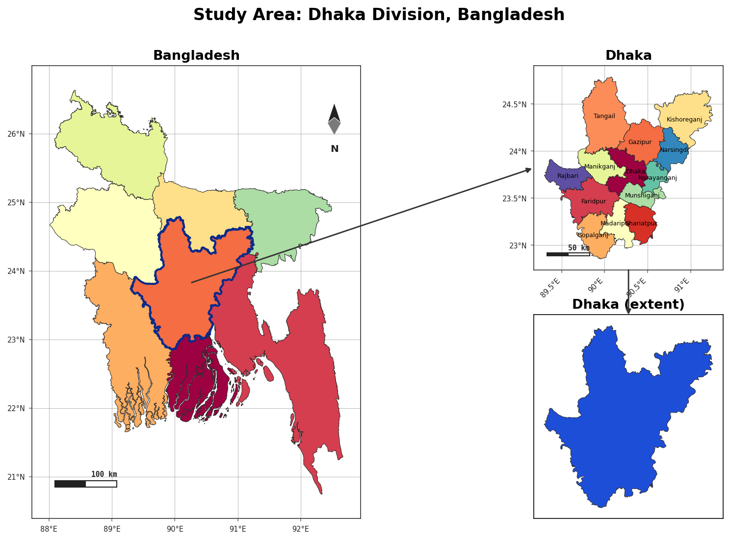
The steps list drives the drill-down: each (level, name) pair narrows the focus. The first
panel is always the whole country; the last panel is the final detail area.
Templates
Pick a layout with template=. agis.TEMPLATES lists them and how many panels each uses:
| Template | Panels | Layout |
|---|---|---|
single |
1 | one map |
two |
2 | a smaller context map + a larger square focus map |
cascade |
3 | two context panels (same size) + one big focus panel |
series |
3 | three uniform panels in a row |
grid |
4 | a 2 × 2 grid |
agis.study_area("Bangladesh", steps=STEPS, template="series")
agis.study_area("Bangladesh", steps=STEPS, template="grid")
Region highlighting
The parent panel highlights the child region. Choose the style:
agis.study_area("Bangladesh", steps=STEPS,
                highlight_style="overlay",   # overlay · rect · circle
                highlight_color="#e63946",
                highlight_alpha=0.30,
                highlight_width=2.0)
overlay— fills the region border with a translucent colour (default)rect— a rectangle around the regioncircle— a circle around the region
Connectors
Lines link each panel to the next. They're fully customizable — or off:
agis.study_area("Bangladesh", steps=STEPS,
                links=True,
                link_color="#1b9aaa",
                link_width=1.6,
                link_style="--",   # any matplotlib line style
                box=True)          # draw the focus box on the parent
Panel sizes
series and grid are uniform by default; cascade and two follow the plan above. Override
any of it:
agis.study_area("Bangladesh", steps=STEPS, template="cascade",
                width_ratios=[1, 2.4], height_ratios=[1, 1.3],
                wspace=0.18, hspace=0.22,
                figsize=(16, 9))
Keep every panel box identical with uniform_panels:
Per-panel decorations
Pass a list to control each panel independently:
agis.study_area("Bangladesh", steps=STEPS, template="cascade",
                graticule=[True, True, False],          # grid off on the focus map
                graticule_interval=[2, 0.5, 0.1],       # degrees, per panel
                north_arrow=[True, False, True],
                scale_bar=True)
Terrain focus panel
terrain=True renders the final panel as Copernicus GLO-30 shaded relief instead of polygons:
Requires pip install "acadgis[terrain]". See Terrain.
Colours
agis.study_area("Bangladesh", steps=STEPS,
                palette="vibrant",       # context panels
                detail_palette="earth",  # focus panel
                cmap="terrain")          # terrain colormap
Hand-drawn overlays with fig.panels
study_area() returns the matplotlib Figure and exposes each map panel on fig.panels, so you
can keep drawing — custom highlights, hand-placed connectors, extra points:
fig = agis.study_area("India", steps=[("state", "Uttarakhand"),
                                      ("district", "Chamoli")],
                      template="cascade", links=False)
axA, axB, axC = fig.panels[:3]

# custom overlay on the second panel
uk = agis.load_boundaries("India", "district", within="Uttarakhand")
uk[uk["NAME_2"] == "Chamoli"].plot(ax=axB, facecolor="#ffd166",
                                   alpha=0.5, edgecolor="#e63946",
                                   linewidth=2.5, zorder=9)

# a hand-placed connector (figure coordinates)
from matplotlib.patches import ConnectionPatch
fig.add_artist(ConnectionPatch(
    xyA=(0.5, 0.0), coordsA=axA.transAxes,
    xyB=(0.5, 1.0), coordsB=axB.transAxes,
    color="#e63946", lw=1.8, zorder=50, clip_on=False))

agis.show()
Coordinate systems: transData = map lon/lat, transAxes = panel 0–1, transFigure = whole figure.
The fluent builder
For step-by-step control there's also the StudyArea builder:
agis.StudyArea("India", context_level="state") \
    .zoom_into("West Bengal", detail_level="district") \
    .figure(suptitle="Study area: West Bengal")
Both produce the same kind of figure — use whichever reads better for your script.