Quickstart

Everything below runs on the bundled offline data — no download needed. Import once:

import acadgis as agis

That single import also gives you agis.plt, agis.np, agis.pd and agis.gpd.

1. Load boundaries by name

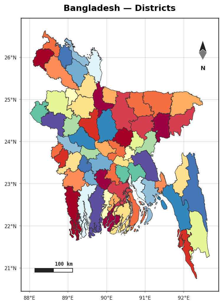
gdf = agis.load_boundaries("Bangladesh", level="district")
dhaka = agis.load_boundaries("Bangladesh", "district", within="Dhaka")

Friendly level names (country, state, district, upazila, …) map to the right GADM level for each country. See Boundaries.

2. A styled map in one call

agis.plot(gdf, palette="spectral", title="Bangladesh — Districts")

3. Choropleth from a spreadsheet — messy names welcome

agis.choropleth(gdf, df, value="incidence",
                palette="magma", scheme="natural_breaks")

Names like Chittagong match Chattogram automatically. See Choropleths.

4. Collected data as graduated symbols

ax = agis.plot(gdf, highlight="Comilla")
agis.points(ax, survey_df, value="value", size_by="value",
            cmap="magma", legend=True)

5. Terrain relief down to a realistic sea

dem = agis.load_dem("Bagrote Valley")
agis.relief(dem, hillshade=True, ocean_color="#cce5f0")

6. The signature multi-panel locator

The fluent builder:

agis.StudyArea("India", context_level="state").zoom_into(
    "West Bengal", detail_level="district").figure()

…or the whole layout in one call with a template:

agis.study_area(
    "Bangladesh",
    steps=[("division", "Dhaka"), ("district", "Madaripur")],
    template="cascade", terrain=True,
)

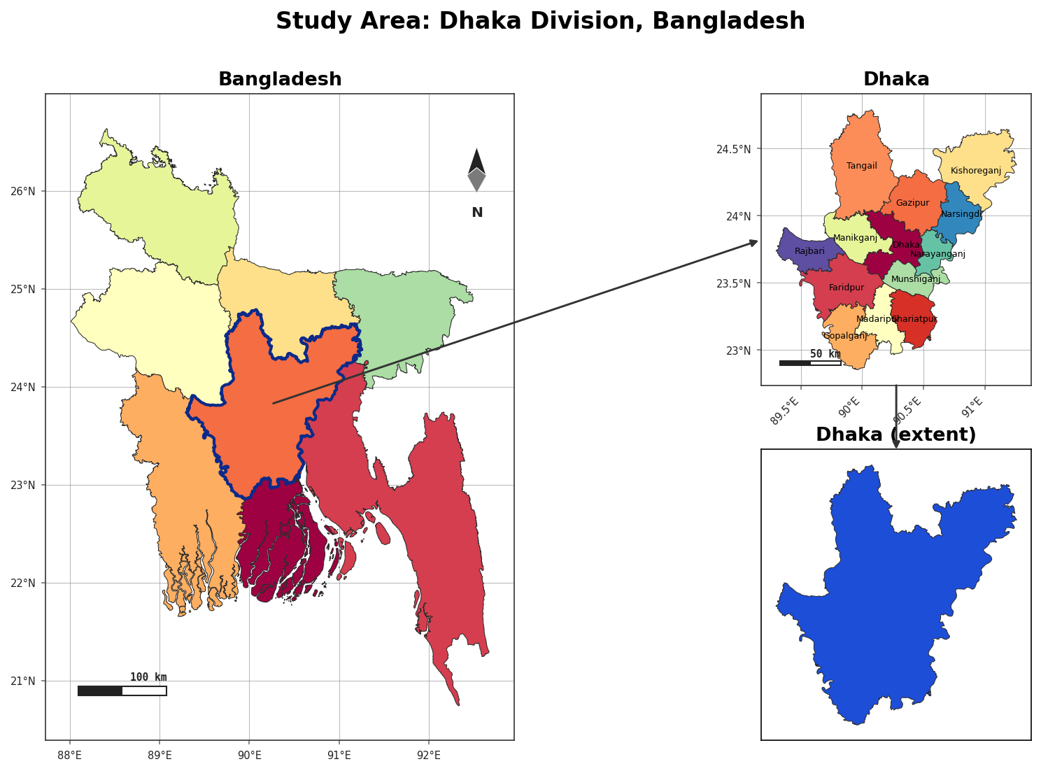
Templates: single · two · cascade · series · grid. See Study-area layouts.

7. Export at any DPI

agis.save("figure.png", dpi=300)   # also .pdf, .svg

---

Next: the User guide covers each feature in depth, or jump to a Tutorial.